Our Hyspex data processing workflow is an adapted version of the workflow established by DLR in 2012. It includes an additional step for correcting the effects of Bidrectional Reflection Distribution Function (BRDF), a phenomenon that partcularly impacts imagery acquired in high-latitude study sites. For ease the processing workflow is presented in four steps:

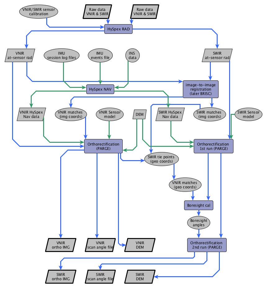Step 1: Image Orthorectification. For quality control we assess general sensor characteristics (eg. spectral smile), sensor calibration and performance issues (eg. striping, data drops), and external conditions during overflight (eg. cloud cover).

Using the HySpex RAD module (part of the software provided by the manufacturer) we apply the laboratory derived calibration coefficients to convert brightness values (DN values) to at-sensor radiance. We then input IMU/GPS data in the Hyspex NAV module, and orthorectify images in the PARGE software using the NAV data, the HySpex sensor model, and a digital elevation model (DEM).

Additionally, we apply boresight calibration during a second PARGE run. The outputs from Step 1 are VNIR and SWIR orthorectified images, scan angle files, and DEMs.

 

Step 2: Generate supercube and DEM derivatives. Next we stack the orthorectified VNIR and SWIR at-sensor radiance images, use the scan angle files from both sensors to generate a mask that includes common image area acquired by both sensors, and clip the stacked images with the mask to generate one large supercube of image data.

Furthermore, we derive slope, aspect, and skyview products from the VNIR and SWIR DEMs, generated in Step 1. These products come in handy for further processing.

 

Step 3: Complete radiometric (including atmospheric and BRDF) corrections. This step brings together several input parameters measured or derived in the earlier steps, into the SPECTRA module.

Atmospheric correction is performed using a radiative transfer-based approach with ATCOR software to convert at-sensor radiance to surface reflectance values. Reliable atmospheric correction of the hyperspectral data requires a DEM and robust parameterization of atmospheric column properties including atmospheric gases (water vapor and oxygen) and aerosol optical thickness (AOT).

The user can supply a high-resolution DEM (if available) or the workflow will use the DEM products generated in Step 2. The DEM products are also used to apply BRDF corrections at this stage. Similarly, the user can provide atmospheric parameters based on atmospheric profiles of the study site (if available), or the processing chain will use a modeled standard atmosphere for the specific geographic region. The output from this step is a data cube corrected for geometric, atmospheric, and BRDF effects.

 

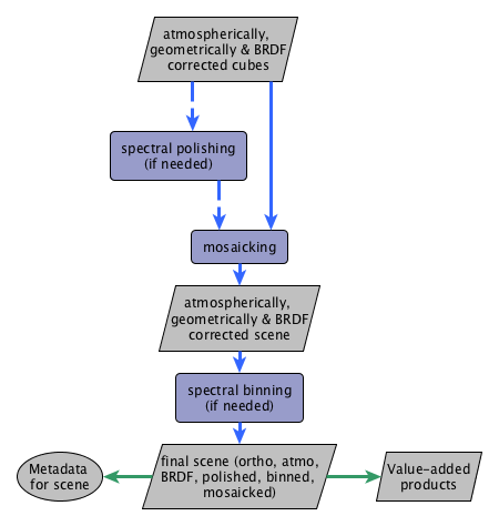Step 4: Spectral polishing, mosaicking, binning. Hyspex data has very narrow spectral bands, and even after optimal corrections for spectral smile and atmospheric effects, the spectral profile may contain artifacts. If required, spectral polishing can be applied to remove such remanent artefacts.

We then mosaic the individual corrected flight lines. To further increase the signal to noise ratio, if the application so demands, we can perform a spectral binning. This dataset is now ready for end-users and for generating higher order products.

Examples of higher order products that the processing automatically generates include leaf area index, NDVI, soil adjusted vegetation index, albedo, and landcover.